Hedging American Put Options with Deep Reinforcement Learning: Training Procedures

Table of Links

1. Abstract

2. Introduction

   Background

   Reinforcement Learning

   Similar Work

3. Methodology

   DRLAgent Design

4. Training Procedures

5. Testing Procedures

6. Results

7. SABR Experiments

8. Conclusions

9. Appendix A

10. References

TRAINING PROCEDURES

Given the design of the state, action, and reward, training a DRL agent to hedge American put options requires the following:

1. The generation of asset price data, used in the DRL agent state and reward.

2. The American put option price, used in the DRL agent reward.

It is noted that counterparty exercise decisions are not considered in training, and training episodes continue past the expected exercise boundary. This is done to ensure that DRL agents experience prices below these boundaries, thereby improving robustness, as there is no guarantee that counterparties will exercise at the expected optimal boundary.

While all DRL agents in this study have the same architecture and hyperparameters, the training procedure differs across two rounds of experiments. The first series of experiments uses MC simulations of a GBM process to generate asset price data, and a second series of experiments uses MC simulations of a calibrated stochastic volatility model as the underlying asset price process.

GBM Experiments: Training Procedures

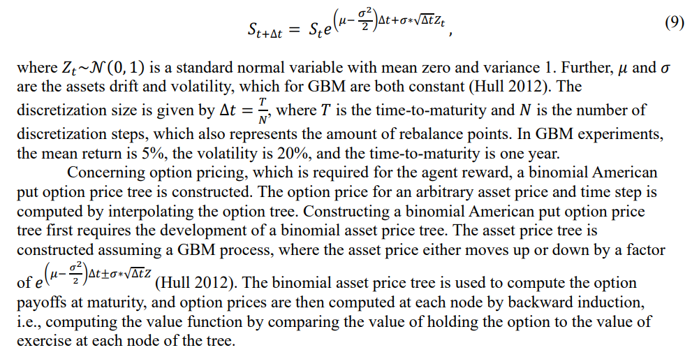
In the GBM experiments, MC paths are simulated as:

Stochastic Volatility Experiments: Training Procedures

In the second round of experiments, MC paths of a stochastic volatility model are simulated. The stochastic volatility model setup is given by:

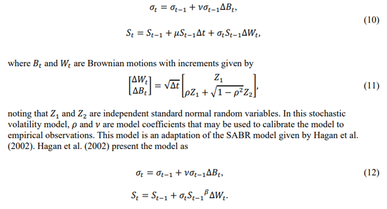
As such, for the model used in this study a non-zero drift term 𝜇 is added, and the 𝛽 parameter is set equal to 1.

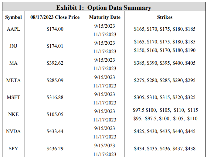
Before calibrating the model to empirical option prices, a preliminary stochastic volatility experiment makes use of arbitrary model coefficients, setting 𝜌 to -0.4, which is reflective of the inverse relationship between asset prices and volatility (leverage effect) (Florescu and Pãsãricã 2009), and 𝜈 to 0.1. The stochastic volatility model is then calibrated to match true market assets. Specifically, given a listed price, maturity date, strike, and thereby an implied volatility, a DRL agent is implemented to hedge this specific option by using a calibrated stochastic volatility model for training. The empirical option data in this study is retrieved from the via the Bloomberg composite option monitor. For 8 symbols, put option prices on August 17th, 2023, for two different maturities (September 15th, 2023, and November 17th, 2023) and five different strikes were retrieved, giving a total of 80 options. Exhibit 1 summarizes the option data. Note that for each of the 80 options, the implied volatility is listed on the option monitor, and the option price is available by computing a mid-price of the bid-ask spread.

For each option, model coefficients 𝜌 and 𝜈 are calibrated by setting the initial volatility to the retrieved implied volatility and minimizing the difference between the option mid-price and the average payoff given by 10000 model generated paths. Specifically, the constrained trustregion optimization algorithm is used. Given a parameter set for each symbol, the model parameters for each symbol are computed by taking an average. Note that the retrieved options are European, so no early exercise is considered when calibrating the model coefficients in this experiment. While the training and testing of the DRL agent considers American style options, model coefficients are calibrated without the exercise boundary, as the construction of said exercise boundary requires calibrated coefficients.

As for option pricing at each time step, recall that GBM experiments use the interpolation of a binomial option tree. However, tree models increase in complexity when considering a stochastic volatility model with two random variables, as the tree now requires a second spatial dimension. Without a binomial tree, American put option prices in this study are computed by leveraging a technique presented by Glau, Mahlstedt, and Potz (2018) that involves approximating the value function at each time-step by a Chebyshev polynomial approximation. Chebyshev approximation involves fitting a series of orthogonal polynomials to a function (Chebyshev 1864). A main advantage to using Chebyshev pricing method for this work is the increased efficiency over a simulation based approach. For example, given an exercise boundary, such as one generated the popular Longstaff-Schwartz Monte Carlo (LSMC) (Longstaff and Schwartz 2001) method, option prices for a given asset price and timestep may be computed by simulating several thousand MC paths of the underlying process to expiry or exercise, and the option price is computed as the average payoff. However, in training an RL agent, simulation-based pricing would add a considerable amount of time to the process, as a new series of simulations is required for each step of training. In this study, with 5000 episodes of 25 steps each, 125,000 sets of simulations would be required, an unnecessary addition to the already time-consuming process of training a neural network. Moreover, it is noted that this Chebyshev method is agnostic to the underlying asset evolution process.

Chebyshev interpolation involves weighing a set of orthogonal interpolating polynomials of increasing order so that their weighted sum approximates a known function between a predetermined upper and lower bound at each time step, which are determined from the extremal excursions of the underlying asset paths. The general Chebyshev process for pricing American options first requires discretizing the computational space from 𝑡0 = 0 to 𝑡𝑁 = 𝑇. Then, the following three-step process ensues:

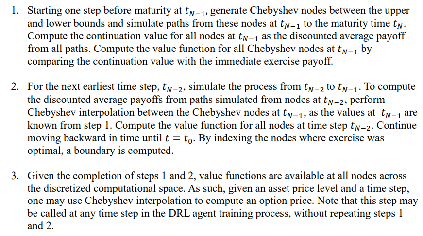
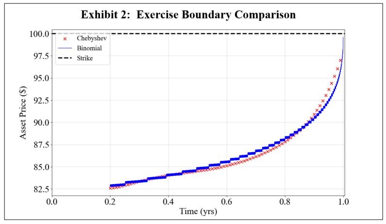
To further exemplify why this Chebyshev method was chosen over LSMC, the reader is directed to Glau, Mahlstedt, and Potz (2018) for a full performance comparison of the Chebyshev and LSMC exercise boundaries. While the Chebyshev method is used for stochastic volatility experiments, the accuracy of the Chebyshev pricing method may be assessed by plotting the Chebyshev exercise boundary for a GBM case where there is a known, true boundary generated by a binomial tree with 5000 nodes. Specifically, consider an at-the-money American put option struck at $100 with a 1-year maturity. Letting the underlying asset follow a GBM process, a comparison of the Chebyshev and binomial boundaries is given in Exhibit 2, and the results show a pronounced agreement between the two methods.